Trend Filtering: what we know and the future
Trend filtering
Trend filtering is an estimator that uses discrete differences to smooth a noisy vector (or more generally, tensor). The method was proposed and computational methods were studied in the 2000’s for data on multidimensional grids. Basically, it takes the general form,
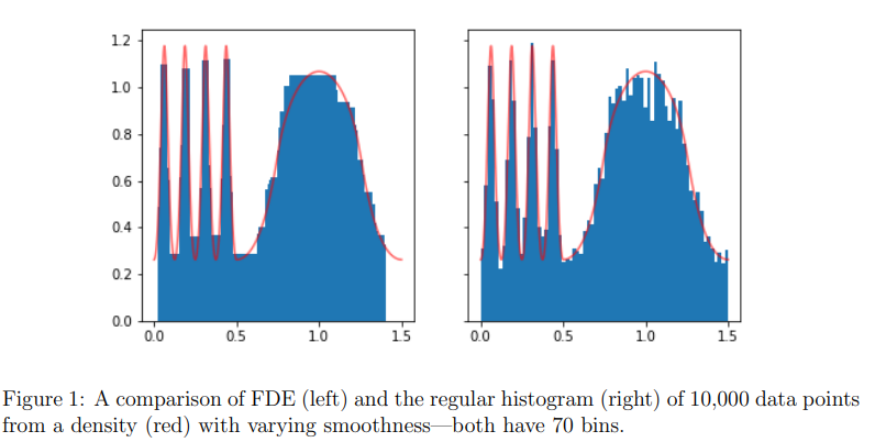
\[\sum_i \ell(\beta_i; y_i) + \lambda \| D^{(k)} \beta \|_1\]where D is a discrete differencing operator. The k is the order, basically, for k of 1 you get piecewise constant signal, and for higher k you get piecewise polynomials. FYI trend filtering with k of 1 is called the fused lasso or total variation denoising (for one of my papers I regrettably tried to rename this the ‘edge lasso’ when applied to graphs). The nice thing about this is that you get automated knot selection, which happens because you are using an L1 penalty. This gives you local adaptivity, which is when your estimator adapts to the local smoothness of the underlying signal. You can use this with most losses, for example, the Poisson loss can give you locally adaptive histograms,
Graph trend filtering
It is pretty straightforward to define the fused lasso (k=1) over graphs, you just let D be the incidence matrix, which turns the penalty into the L1 of the difference across edges of the graph. For higher order graphs, we had to make some choices, and what we settled on is
\[D^{(k+1)} = \Big\{ \begin{array}{ll} D^\top D^{(k)},& k~{\rm odd} \\ D D^{(k)}, & k~{\rm even} \end{array}.\]This has the desired local adaptivity property, as evidenced by this example over the Allegheny county zip codes (it varies the smoothness locally) which are connected based on direct proximity:
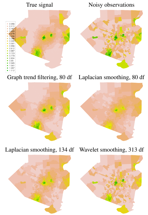
Image courtesy of Ryan Tibshirani
What we know
So after years of studying trend filtering we have some things that we do know (about theory). First, I would like to call out two types of results,
-
L0 rates: these are results that assume that true signal satisfies a sparsity assumption, that there are only s non-zero discrete derivatives. Typically, the hope is to recover the standard ‘parametric’ rates of the lasso, \(\| \hat \beta - \beta_0 \|^2 \lesssim s~{\rm plog} n\) for some choice of tuning parameter and \(\beta_0\) is the true signal.
-
L1 rates: these are results that assume that the true signal have only bounded L1 norm (total variation), i.e. \(\| D \beta \|_1\) is bounded. Typically, here you show that \(\| \hat \beta - \beta_0 \|^2 \lesssim n^\alpha~{\rm plog} n\) for some choice of tuning parameter.
The problem with 1, is that you can get the parametric rates regardless of the graph structure (as long as it is connected) for the fused lasso. We showed this with the depth-first-search (DFS) wavelets (at least for the fused lasso) in this paper. Basically, 1 only requires a tree structure and not a more highly connected graph structure. It is substantially harder to show this for higher order trend filtering, even in 1 dimension (see this paper by Guntuboyina et al. and our prior work), and there is a loss in log factors if you go with the DFS wavelet approach. The satisfying thing about results of type 2 is that the rate parameter \(\alpha\) depends on the graph structure, and smaller typically means a more connected graph. For this reason, I have focused on this type of result.
There is a third type of result, which gives you exact reconstruction of the region where you have polynomial structure. I attempted this in this paper, but the conditions are ridiculous. I believe that this is insurmountable, and I provide some evidence.
So, what do we know?
- Rates for Gaussian noise, grid graphs (Veeru Sadhanala’s thesis, this paper)
- Rates for density estimation, in 1 dimension (and ‘geometric graphs’) with k=1 (fused lasso).
- A base rate for all connected graphs with k=1, spoiler, it is the same as the 1D fused lasso \(n^{1/3}\).
- A tool, called eigenvector incoherence, for analyzing any order over any graph that is tight in some cases.
- A specialized result for k=1, nearest neighbor graphs, turns out that the rate is the same for grids on the intrinsic dimension of the manifold.
- Rates for additive trend filtering models
- Lower bounds for multidimensional trend filtering
Future work (that I probably will not pursue myself)
So there is a lot that we don’t know, here are some thoughts.
- The eigenvector incoherence tool gives us a method for analyzing any graph, but it is very opaque. It would be better if we could relate the rates to a functional of the graph that is more interpretable and easier to analyze.
- General exponential families are mostly wide open.
- Rates for trend filtering in high dimensions under strong sparsity assumptions.
- There are strange behaviors for higher order GTF on point clouds in multiple dimensions, particularly at the boundaries of the support. For \(k=1\) this goes away, but at higher order, we need to modify GTF. Our best guess at the ideal approach is to come up with a fine spline basis and then come up with the trend filtering penalty on this.